We’re back to Kaggle competitions. This time we will attempt to predict advertised salaries from job ads and of course beat the benchmark. The benchmark is, as usual, a random forest result. For starters, we’ll use a linear model without much preprocessing. Will it be enough?

A linear model better than a random forest - how so? Well, to train a random forest on data this big, the benchmark code extracts only 100 most common words as features, and we will use all. This approach is similiar to the one we applied in Merck challenge. More data beats a cleverer algorithm, especially when a cleverer algorithm is unable to handle all of data (on your machine, anyway).

The competition is about predicting salaries from job adverts. Of course the figures usually appear in the text, so they were removed. An error metric is mean absolute error (MAE) - how refreshing to see so intuitive one.

The data for Job salary prediction consists of several columns, which are mostly either text or categorical. For text features, we will use a bag of words representation. Then we will feed everything to Vowpal Wabbit, which seems to be quite good at handling this type of thing.

Refer to Predicting closed questions on Stack Overflow for basics of using Vowpal Wabbit.

Code for predicting advertised salaries is available at Github.

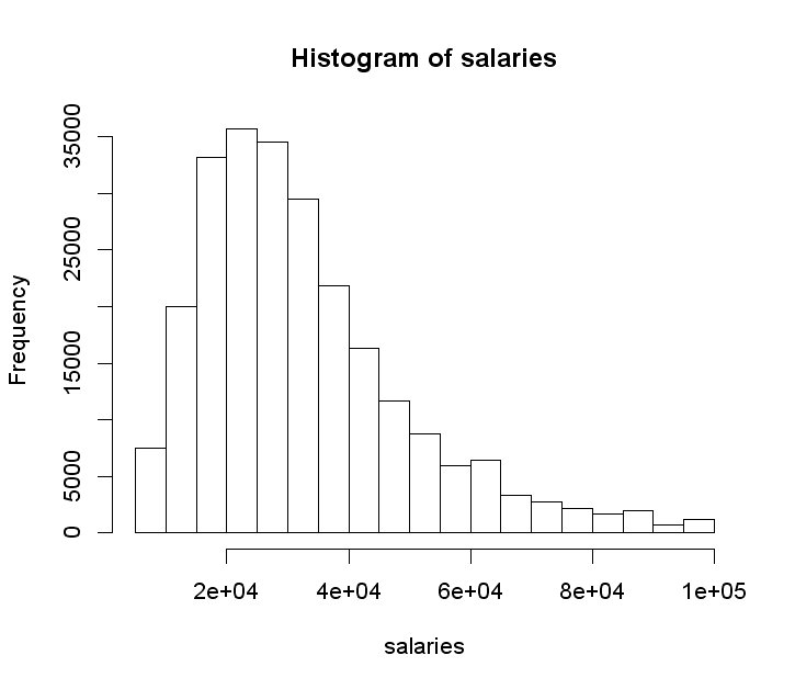
The distribution of salaries

UPDATE: As Dang Ha The Hien points out in the comments, linear regression actually assumes the errors (residuals) are normally distributed. The transformation of the dependent variable might help achieve normality of the residuals:

I believe that for dependent variables which are restricted to be positive, e.g. salary, interest, rate of return…, we usually need some kind of transformation (usually log) because the variance of errors will increase when the value of dependent variable increases. For example in your ads salary problem, if your model predicts an ads’s salary is 100k$, the 20k$ error is more likely to happen than when you predict an ads’s salary is 30k$. Generally, in these cases, the standard deviations of the residual distributions increase when the dependent variables increase.

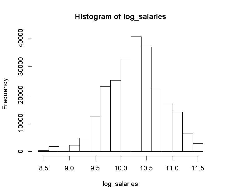
VW, being a linear learner, probably expects the target variable residuals to have a normal distribution. We checked empirically ;) Therefore, it is important to log transform salaries, because the original distribution is skewed:

After the transform, we get something closer to a bell curve. The right is side chopped off on this plot for some reason, in reality the upper range is 12.2.

Another option would be to take a square root of salaries:

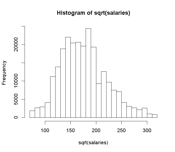
Validation shows that the log transform works better in this case.

Validation

For validation purposes, we convert a training set file to a VW format, then split it randomly into train and validation sets (95% train, 5% validation). The main parameter to tune is a number of passes over the data, as usually one is not enough for optimal results. 20 passes produces a lowest validation MAE.

We don’t expect other hyperparams to matter that much, but it might be worth tweaking the bits -b a little, or maybe add some explicit regularization. By explicit we mean that limiting a number of passes works as regularization.

Data preparation

We will refer to the original Validation.csv file as the test file, because that’s what it is at the moment (there’s no labels in there).

To produce a submission file we need to prepare the data a little bit, namely convert it to VW format with 2vw.py. Here’s a snippet describing what we do with the columns:

target_col = 'SalaryNormalized'
cols2tokenize = [ 'Title', 'FullDescription', 'LocationRaw' ]
cols2binarize = [ 'LocationNormalized', 'ContractType', 'ContractTime', 
    'Company', 'Category', 'SourceName' ]
cols2drop = [  'SalaryRaw' ]

By binarizing we mean encoding categorical variables as one-hot vectors and expressing them in libsvm format, that is, by the index of the one among zeros. This sounds more complicated than it is. Example: 0 0 0 1 0 becomes 4:1, or just 4.

You could just give VW a value of a categorical variable with spaces removed to achieve the same effect, but we had the binarizing code handy. The advantage of employing it (it’s a post about job salaries, isn’t it?) is that the output file is smaller.

The disadvantage is that we need to convert training and test files together, that is combine them, convert, and then split back. Otherwise train and test feature indices won’t match.

To combine the files, we need to add dummy salary columns to the test file, so that the columns in both files match. We do this using add_dummy_salaries.py script:

add_dummy_salaries.py Valid.csv Valid_with_dummy_salaries.csv

If you’re on Unix, you concatenate files:

cat Train.csv Valid_with_dummy_salaries.csv > train_plus_valid.csv

On Windows, it’s

copy Train.csv+Valid_with_dummy_salaries.csv train_plus_valid.csv.

Then convert:

2vw.py train_plus_valid.csv train_plus_valid.vw

To split the files back, we use first.py script like this: first.py train_plus_valid.vw train.vw 244768 first.py train_plus_valid.vw test.vw 999999999 244768

The third argument to first.py is a number of lines to write to the output file (those nines are just a big number, or a way of saying “till the end”). The script starts with the first line, or the line specified by the fourth argument, if it is there.

Running VW and the result

Now let’s run VW:

vw -d data/train.vw -c -f model --passes 20 vw -t -d data/test.vw -c -i model -p data/p.txt

Predictions come out on the log scale, so the last step is to convert them back. We do this with unlog_predictions.r.

The result is pretty good:

The remarkable thing is that the test score is almost the same as the validation score, which was 7149. This means that the train and test files come from the same distribution - a good thing for predicting.

UPDATE: Kaggle released a revised data set, the new score is 6734.