Pandas is Python software for data manipulation. We show that some rather simple analytics allow us to attain a reasonable score in an interesting Kaggle competition. While doing that, we look at analogies between Pandas and SQL, a standard in relational databases.
Pandas provides functionality similar to R’s data frame. Data frames are containers for tabular data, including both numbers and strings. Unfortunately, the library is pretty complicated and unintuitive. It’s the kind of software you constanly find yourself referring to Stack Overflow with. Therefore it would be nice to have a mental model of how it works and what to expect of it.
We discovered this model listening to a talk by Wes McKinney, the creator of Pandas. He said that the library started as a replacement for doing analytics in SQL.
SQL is a language used for moving data in and out of relational databases such as MySQL, Oracle, PostgreSQL, SQLite etc. It has strong theoretical base called relational algebra and is pretty easy to read and write once you get the hang of it.
These days you don’t hear that much about SQL because proven, reliable and mature technology is not a news material. SQL is like Unix: it’s a backbone in its domain.
Trying out SQL
Want to try SQL? One of the easiest ways is to use SQLite. Contrary to other databases, it doesn’t require installation and uses flat files as storage. You’d suspect it’s much slower or primitive, but no. In fact, it’s one of the finest pieces of software we have seen. It’s small, fast and reliable, and has an extensive test suite. The users include Airbus, Apple, Bosch and a number of other well-know companies.
Pandas can read and write to and from databases, so we can create a database in a few lines of code:
import pandas as pd
import sqlite3

train_file = 'data/train.csv'
db_file = 'data/sales.sqlite'

train = pd.read_csv( train_file )
conn = sqlite3.connect( db_file )

train.to_sql( 'train', conn, index = False, if_exists = 'replace' )
After that, you can use Pandas or one of the available managers to connect to the database and execute queries.
The competition
Pandas’ SQL heritage shows, once you know what to look for. If you’re familiar with SQL, it makes using Pandas easier. We’ll show some operations that could be done with either. For demonstration, we’ll use the data from the Rossmann Store Sales competition.
More often that not, Kaggle competitions have quirks. For example: dirty data, a strange evaluation metric, test set markedly different from a train set, difficulty in constructing a validation set, label leakage, few data points, and so on.
One might consider some of these interesting or spicy; the other just spoil the fun. The fact is, rarely do you come across a contest where you can just go and apply some supervised methods off the bat, without wrestling with superfluous problems. The Rossman competition is a rare exception.
The point is to predict sales in about a thousand stores across Germany. There are roughly million training points and 40k testing points. The training set spans January 2013 through June 2015, and the test set the next three months in 2015.
The data is clean and nice, prepared with German solidity. There are some non-standard things to consider, but they are mostly of the good kind.
We’re dealing with a time dimension. This is a very common problem. How to address it? One can pretend the data is static and use feature engineering to account for time. As the features we could have, for example, binary indicators for the day of week (already provided), the month, perhaps the year. Another possibility is to come up with a model inherently capable of dealing with time series.
Evaluation metric is RMSE, but computed on relative error. For example, when you predict zero for non-zero sales, the error value is one. When you predict twice the actual sales, the error also will be one. In effect, this metric doesn’t favour big stores over small ones, as raw RMSE would.
Shop ID is a categorical variable, and relatively high-dimensional. This might make using our first choice, tree ensembles, difficult. Solution? Employ a method able to deal both with high dimensionality and feature interactions (because we need them). Factorization machines is one such method. Another option: transform data to a lower-dim representation.
Besides usual prices for the 1st, 2nd and 3rd place, there’s an additional prize for the team whose methodology Rossman will choose to implement. We consider this a very welcome improvement, as it addresses some issues with Kaggle we raised a while ago.
Sales
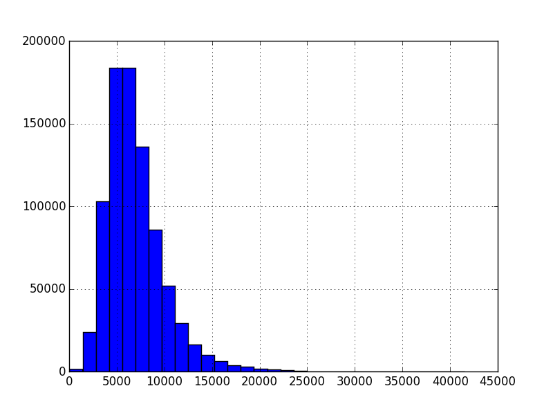
Let’s look at a histogram of sales, excluding zeros:
train.loc[train.Sales > 0, 'Sales'].hist( bins = 30 )
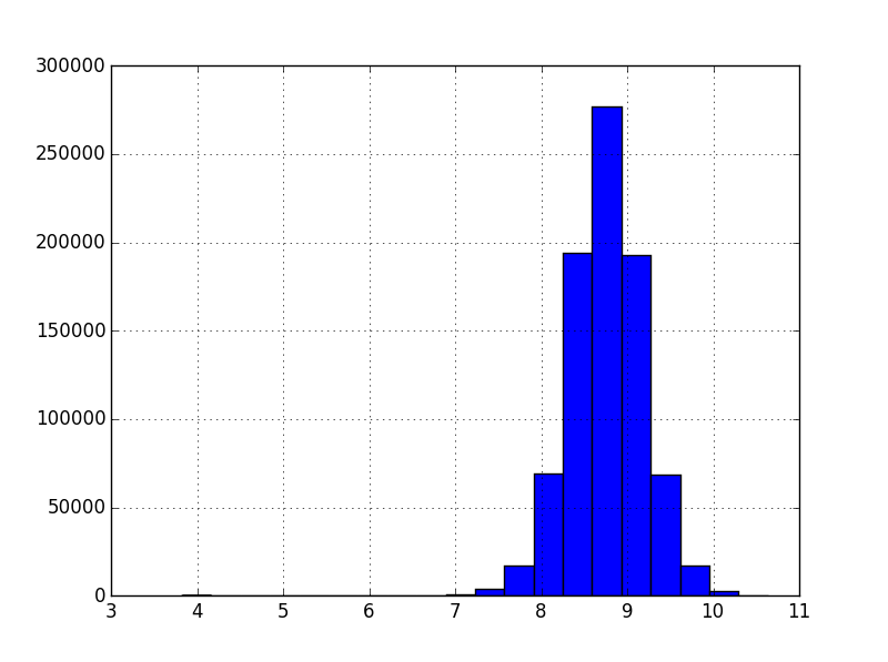
Should we need normality, we can apply the log-transform:
np.log( train.loc[train.Sales > 0, 'Sales'] ).hist( bins = 20 )
The benchmark
The benchmark for the competition predicts sales for any given store as a median of sales from all stores on the same day of the week. This means we GROUP BY the day of the week:
medians_by_day = train.groupby( ['DayOfWeek'] )['Sales'].median()
The result:
In [1]: medians_by_day
Out[1]:
DayOfWeek
1    7310
2    6463
3    6133
4    6020
5    6434
6    5410
7       0
Name: Sales, dtype: int64
Here’s the same thing in SQL:
SELECT DayOfWeek, MEDIAN( Sales ) FROM train GROUP BY DayOfWeek
We prefer the median over the mean because of the metric. Unfortunately, MEDIAN function seems to be missing from the popular databases, so we have to stick with the mean for the purpose of this demonstration:
SELECT DayOfWeek, AVG( Sales ) FROM train GROUP BY DayOfWeek
By convention, we use uppercase for SQL keywords, even though they are case-insensitive. We’re selecting from a table called train, so we’d also have test, just like train and test files. Since both contain data with the same structure, in real life they would probably be in one table, but let’s play with two for the sake of analogy.
Removing days with zero sales
The organizers decided leave in the days where stores were closed, probably to keep the dates continuous. The sales for these days were zero. Currently we’re not taking this into account, but we probably should:
medians_by_day_open = train.groupby( ['DayOfWeek', 'Open'] )['Sales'].median()

In [3]: medians_by_day_open
Out[3]:
DayOfWeek  Open
1          0          0
           1       7539
2          0          0
           1       6502
3          0          0
           1       6210
4          0          0
           1       6246
5          0          0
           1       6580
6          0          0
           1       5425
7          0          0
           1       6876
Name: Sales, dtype: int64
By the way, medians_by_day_open returned is a series:
In [4]: type( medians_by_day_open )
Out[4]: pandas.core.series.Series
We’d get the median for Tuesday/Open the following way:
In [5]: medians_by_day_open[2][1]
Out[5]: 6502
Note how these numbers are bigger than medians by day only. We get a better estimate by excluding “closed” days, and the easiest way to do this is removing them from the train set:
train = train.loc[train.Sales > 0]

DELETE FROM train WHERE Sales = 0
Just for completeness, there seems to be a few days where a store was open but no sales occured:
In [6]: len( train[( train.Open ) & ( train.Sales == 0 )] )
Out[6]: 54
Beating the benchmark
The obvious way to improve on the benchmark is to group not only by day of week, but also by a store. Running the query in Pandas:
query = 'SELECT DayOfWeek, Store, AVG( Sales ) AS AvgSales FROM train
    GROUP BY DayOfWeek, Store'
res = pd.read_sql( query, conn )

res.head()
Out[2]:
   DayOfWeek  Store      AvgSales
0          1      1   4946.119403
1          1      2   5790.522388
2          1      3   7965.029851
3          1      4  10365.686567
4          1      5   5834.880597
Note that we can give an alias to AVG( Sales ), which is not a very good name for a column, SELECTing AS.
Even better, we can include other fields, for example Promo. We have enough data to get medians for every possible combination of these three variables.
medians = train.groupby( ['DayOfWeek', 'Store', 'Promo'] )['Sales'].median()
medians = medians.reset_index()
reset_index() converts medians from a series to a data frame.
In SQL, we would store the computed means for further use in a so called view. A view is like a virtual table: it shows results from a SELECT query.
CREATE VIEW means AS
    SELECT DayOfWeek, Store, Promo, AVG( Sales ) AS AvgSales FROM train
    GROUP BY DayOfWeek, Store, Promo
Merging tables
Data for machine learning quite often comes from relational databases. The tools typically expect 2D data: a table or a matrix. On the other hand, in a database you may have it spread over multiple tables, because it’s more natural to store information that way. For example, there may be one table called sales which contains store ID, date and sales on that day. Another table, stores would contain store data.
If you’d like to use stores info for predicting sales, you need to merge those two tables so that every sale row contains info about the relevant store. Note that the same piece of store data will repeat across many rows. That’s why it’s in the separate table in the first place.
For now, we have the medians/means and want to produce predictions for the test set. Accordingly, there are two data frames, or tables: test and medians/means. For each row in test, we’d like to pull an appropriate median. This could be done with a loop, or with an apply() function, but there’s a better way.
test2 = pd.merge( test, medians, on = ['DayOfWeek', 'Store', 'Promo'], how = 'left' )
This will take the Sales column from medians and put it in test so that Sales match DayOfWeek, Store and Promo in test. The operation is known as a JOIN.
SELECT test.*, means.AvgSales AS Sales FROM test LEFT JOIN means ON (
    test.DayOfWeek = means.DayOfWeek
    AND test.Store = means.Store
    AND test.Promo = means.Promo )
You see that SQL can be a bit verbose.
LEFT JOIN means that we treat the left table (test) as primary: if there’s a row in the left table but no corresponding row to join in the right table, we still keep the row in the results. Sales will be NULL in that case. Contrast this with the default INNER JOIN, where we would discard the row. We want to keep all rows in test, that’s why we use a left join. The resulting frame should have as many rows as the original test:
assert( len( test2 ) == len( test ))
Conclusion
All that is left is saving the predictions to a file.
test2[[ 'Id', 'Sales' ]].to_csv( output_file, index = False )
The benchmark scores about 0.19, our solution 0.14, the leaders at the time of writing 0.10.
The script is available on GitHub and at Kaggle Scripts. Did you know that you can run your scripts on Kaggle servers? There are some catches, however. One, the script gets released under Apache license and you can’t delete it. Two, it can run for at most 20 minutes.
If you want more on the subject matter, Greg Reda has an article (and a talk) on translating SQL to Pandas, as well as a general Pandas tutorial. This Pandas + SQLite tutorial digs deeper.